Q: How accurate is Google Flu Trends?

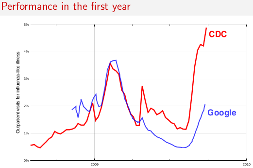
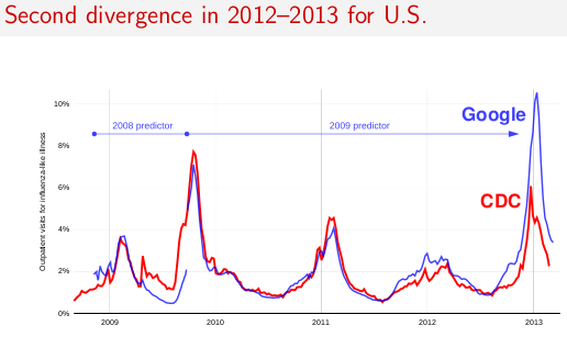
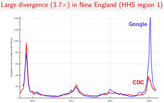
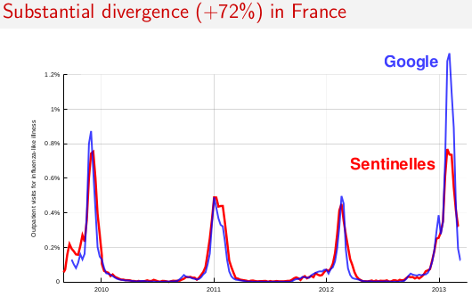
Update March 14, 2013: In 2012–13, Google Flu Trends did not successfully track the target flu indexes in the U.S., France, or Japan. Here are my slides from a talk at the Children's Health Informatics Program (March 14, 2013).

Why this happened is a mystery. Google has said they will present their own view some time this fall. I think the divergence suggests that one needs to be careful about trusting these kinds of machine-generated estimators, even when they work well for three years in a row. It can be hard to predict when they will fall down. (And without an underlying index that is still measured, you might never know when it has stopped working.)

I did an interview with WBUR's CommonHealth blog in January and again in February, and spoke on the radio in January.

---

Q: The probability of success in each of a series of independent trials is constant. How can a 95% confidence interval for this proportion be obtained?

This is called the "binomial confidence interval," and there are a few solutions. Wikipedia discusses this here: Binomial proportion confidence interval

Q: Event A has a probability of 70% of happening within the year and event B, 40%. The events are independent and uniformly distributed through the year. What is the probability that they will occur within 3 months of each other?

There is more than one way to answer this question!

The ambiguity comes down to exactly how we interpret the statement that "Events A and B are uniformly distributed across the year."

FIrst interpretation: Events A and B are produced by a memoryless process with uniform hazard function. Every day, we wake up and Event A has a certain uniform probability of happening that day, the same as every other day. Event B is independent and has its own uniform probability of happening that day. If the event doesn't happen, we go to bed and wake up the next day, and it's the exact same story, with the same probabilities, all over again, just like "Groundhog Day."

Q: Do the odds in a horse race add up to more than 100%?

It doesn't quite make sense to sum odds. But if we talk about converting the odds into the probabilities of each horse's winning, then yes, they do add to more than 100% -- because the house takes more than 16% of every dollar bet!

For example, let's say we had two horses in a race, equally favored to win. A "fair" race chart, with no house take, would give each horse 1:1 odds against winning -- meaning a successful $1 bet will pay back a total of $2. The probability that corresponds to 1:1 odds is 1/(1+1), or 50% -- and two of these sum to 100%. Say you want to be guaranteed to walk away with $1. Then you need to bet 1/2 dollar on each horse. Exactly one horse will win (paying off 1:1, so you'll get a dollar back), so you will break even.

In reality, the odds won't be 1:1 for each horse. It will be something like 2:3 odds for each horse, meaning a successful $3 bet will pay back a total of $5. The probability that corresponds to 2:3 odds is 3/5, or 60%. Two of these sum to 120%! Say you want to be guaranteed to walk away with $5. Then you must bet $3 on the first horse, and $3 on the second horse. You've bet $6 to be assured of winning $5 -- the house has taken 16.7%.

We can see this if you look at the chart from yesterday's running of the Kentucky Derby (http://www1.drf.com/tc/kentuckyderby/2011/pdf/2011-kentucky-derby-chart.pdf ):

The race went off like this:

• Animal Kingdom, 20.90 (odds $1)
• Nehro, 8.50
• Mucho Mucho Man, 9.30
• Shackleford, 23.10
• Master of Hounds, 16.80
• Santiva, 34.70
• Brilliant Speed, 27.90
• Dialed In, 5.20
• Pants On Fire, 8.10
• Twice the Appeal, 11.90
• Soldat, 11.90
• Stay Thirsty, 17.20
• Derby Kitten, 36.30
• Decisive Moment, 39.30
• Archarcharch, 12.50
• Midnight Interlude, 9.60
• Twinspired, 32.90
• Watch Me Go, 33.60
• Comma to the Top, 35.80

Let's say on each horse we made a bet "to win" in the amount of what it took to be assured of walking away with $1. Exactly one bet will succeed, so the amount we need to bet is the reciprocal of one plus the odds. (E.g. if the odds are 9.60 against 1, we can bet 1/10.60 dollars to receive $1 if it's a success.)

The total we need to bet is

1/21.90 + 1/9.50 + 1/10.30 + 1/24.10 + 1/17.80 + 1/35.70 + 1/28.90 + 1/6.20 + 1/9.10 + 1/12.90 + 1/12.90 + 1/18.20 + 1/37.30 + 1/40.30 + 1/13.50 + 1/10.60 + 1/33.90 + 1/34.60 + 1/36.80 = 1.195...

So it takes about $1.20 to be assured of walking away with exactly $1. The house is taking about 16%.

(To be fair, the house is not just one house -- OTB facilities take a cut, etc. etc. But from the perspective of the gambler, the house advantage in horseracing is much higher than even the worst casino games.)

Q: In what ways are the US News & World Report rankings for colleges flawed?

About a quarter of the U.S. News formula is an opinion poll of university administrators (presidents, provosts and deans) and high school college counselors about their views on the reputations of the colleges.

One criticism would be, does this really speak highly for the validity of the results, when 23% of the result comes from administrators at competing universities and high school employees? Does a 45-year-old guidance counselor at Evanston high school or a 60-year-old dean at the University of Chicago really have any idea whether you'll get a better undergraduate education at Stanford, Harvard, Penn or Yale if you go there in 2011?

And, of course, can a national university really have a single, unitary reputation score? Surely the kind of student who would thrive at Caltech (the #1 school in the country a decade ago, despite offering no BA degree) is not the same as the student who would thrive studying medieval literature at Yale.

But #2, like all components of the U.S. News formula, there is no margin of error on the results of the opinion poll! The rankings are calculated as if every input -- the competitor and high-school employee view of a school's "reputation," its graduation rate, the average class size -- were absolutely certain. That is not so. 

In addition to statistical error, there's also a substantial systematic error in some of the parameters -- e.g. the "average class size" has a lot of slop in what you count as a class (just lectures? lectures and discussion sections? lectures, discussion sessions, and tutorials?). So does the graduation rate, etc. These figures should have error bars on them too.

I have discussed this briefly with Bob Morse, the guy at U.S. News who calculates the rankings, but he wasn't receptive to the idea that they should put appropriate error bars on all the inputs and propagate the uncertainty to the outputs, marking statistical ties as appropriate. (I suspect these statistical ties might cross substantial swaths of the final rankings, which may partly explain why U.S. News wouldn't be excited to try to sell magazines with that technique -- who wants to announce a nine-way tie for 1st place?) His position was that they assume the data coming from the schools is right, and they don't waste time worrying about what the rankings would be if the supplied figures weren't right.

Q: What is the difference between Bayesian and frequentist statistics?

Mathematically speaking, frequentist and Bayesian methods differ in what they care about, and the kind of errors they're willing to accept.

Generally speaking, frequentist approaches posit that the world is one way (e.g., a parameter has one particular true value), and try to conduct experiments whose resulting conclusion -- no matter the true value of the parameter -- will be correct with at least some minimum probability.

As a result, to express uncertainty in our knowledge after an experiment, the frequentist approach uses a "confidence interval" -- a range of values designed to include the true value of the parameter with some minimum probability, say 95%. A frequentist will design the experiment and 95% confidence interval procedure so that out of every 100 experiments run start to finish, at least 95 of the resulting confidence intervals will be expected to include the true value of the parameter. The other 5 might be slightly wrong, or they might be complete nonsense -- formally speaking that's ok as far as the approach is concerned, as long as 95 out of 100 inferences are correct. (Of course we would prefer them to be slightly wrong, not total nonsense.)

Bayesian approaches formulate the problem differently. Instead of saying the parameter simply has one (unknown) true value, a Bayesian method says the parameter's value is fixed but has been chosen from some probability distribution -- known as the prior probability distribution. (Another way to say that is that before taking any measurements, the Bayesian assigns a probability distribution, which they call a belief state, on what the true value of the parameter happens to be.) This "prior" might be known (imagine trying to estimate the size of a truck, if we know the overall distribution of truck sizes from the DMV) or it might be an assumption drawn out of thin air. The Bayesian inference is simpler -- we collect some data, and then calculate the probability of different values of the parameter GIVEN the data. This new probability distribution is called the "a posteriori probability" or simply the "posterior." Bayesian approaches can summarize their uncertainty by giving a range of values on the posterior probability distribution that includes 95% of the probability -- this is called a "95% credibility interval."

A Bayesian partisan might criticize the frequentist confidence interval like this: "So what if 95 out of 100 experiments yield a confidence interval that includes the true value? I don't care about 99 experiments I DIDN'T DO; I care about this experiment I DID DO. Your rule allows 5 out of the 100 to be complete nonsense [negative values, impossible values] as long as the other 95 are correct; that's ridiculous."

A frequentist die-hard might criticize the Bayesian credibility interval like this: "So what if 95% of the posterior probability is included in this range? What if the true value is, say, 0.37? If it is, then your method, run start to finish, will be WRONG 75% of the time. Your response is, 'Oh well, that's ok because according to the prior it's very rare that the value is 0.37,' and that may be so, but I want a method that works for ANY possible value of the parameter. I don't care about 99 values of the parameter that IT DOESN'T HAVE; I care about the one true value IT DOES HAVE. Oh also, by the way, your answers are only correct if the prior is correct. If you just pull it out of thin air because it feels right, you can be way off."

In a sense both of these partisans are correct in their criticisms of each others' methods, but I would urge you to think mathematically about the distinction. There don't need to be Bayesians and frequentists any more than there are realnumberists and integeristos; there are different kinds of methods that apply math to calculate different things. This is a complex subject with a lot of sides to it, of which these examples are a tiny part -- books on Bayesian analysis could fill many bookshelves, not to mention classical statistics, which would fill a whole library.

------------

Here's an extended example that shows the difference precisely in a discrete example.

When I was a child my mother used to occasionally surprise me by ordering a jar of chocolate-chip cookies to be delivered by mail. The delivery company stocked four different kinds of cookie jars -- type A, type B, type C, and type D, and they were all on the same truck and you were never sure what type you would get. Each jar had exactly 100 cookies, but the feature that distinguished the different cookie jars was their respective distributions of chocolate chips per cookie. If you reached into a jar and took out a single cookie uniformly at random, these are the probability distributions you would get on the number of chips:

A type-A cookie jar, for example, has 70 cookies with two chips each, and no cookies with four chips or more! A type-D cookie jar has 70 cookies with one chip each. Notice how each vertical column is a probability mass function -- the conditional probability of the number of chips you'd get, given that the jar = A, or B, or C, or D, and each column sums to 100.

I used to love to play a game as soon as the deliveryman dropped off my new cookie jar. I'd pull one single cookie at random from the jar, count the chips on the cookie, and try to express my uncertainty -- at the 70% level -- of which jars it could be. Thus it's the identity of the jar (A, B, C or D) that is the value of the parameter being estimated. The number of chips (0, 1, 2, 3 or 4) is the outcome or the observation or the sample.

Originally I played this game using a frequentist, 70% confidence interval. Such an interval needs to make sure that no matter the true value of the parameter, meaning no matter which cookie jar I got, the interval would cover that true value with at least 70% probability.

An interval, of course, is a function that relates an outcome (a row) to a set of values of the parameter (a set of columns). But to construct the confidence interval and guarantee 70% coverage, we need to work "vertically" -- looking at each column in turn, and making sure that 70% of the probability mass function is covered so that 70% of the time, that column's identity will be part of the interval that results. Remember that it's the vertical columns that form a p.m.f.

So after doing that procedure, I ended up with these intervals:

For example, if the number of chips on the cookie I draw is 1, my confidence interval will be {B,C,D}. If the number is 4, my confidence interval will be {B,C}. Notice that since each column sums to 70% or greater, then no matter which column we are truly in (no matter which jar the deliveryman dropped off), the interval resulting from this procedure will include the correct jar with at least 70% probability.

Notice also that the procedure I followed in constructing the intervals had some discretion. In the column for type-B, I could have just as easily made sure that the intervals that included B would be 0,1,2,3 instead of 1,2,3,4. That would have resulted in 75% coverage for type-B jars (12+19+24+20), still meeting the lower bound of 70%.

My sister Bayesia thought this approach was crazy, though. "You have to consider the deliverman as part of the system," she said. "Let's treat the identity of the jar as a random variable itself, and let's assume that the deliverman chooses among them uniformly -- meaning he has all four on his truck, and when he gets to our house he picks one at random, each with uniform probability."

"With that assumption, now let's look at the joint probabilities of the whole event -- the jar type and the number of chips you draw from your first cookie," she said, drawing the following table:

Notice that the whole table is now a probability mass function -- meaning the whole table sums to 100%.

"Ok," I said, "where are you headed with this?"

"You've been looking at the conditional probability of the number of chips, given the jar," said Bayesia. "That's all wrong! What you really care about is the conditional probability of which jar it is, given the number of chips on the cookie! Your 70% interval should simply include the list jars that, in total, have 70% probability of being the true jar. Isn't that a lot simpler and more intuitive?"

"Sure, but how do we calculate that?" I asked.

"Let's say we know that you got 3 chips. Then we can ignore all the other rows in the table, and simply treat that row as a probability mass function. We'll need to scale up the probabilities proportionately so each row sums to 100, though." 

She did:

"Notice how each row is now a p.m.f., and sums to 100%. We've flipped the conditional probability from what you started with -- now it's the probability of the man having dropped off a certain jar, given the number of chips on the first cookie."

"Interesting," I said. "So now we just circle enough jars in each row to get up to 70% probability?" We did just that, making these credibility intervals:

Each interval includes a set of jars that, a posteriori, sum to 70% probability of being the true jar.

"Well, hang on," I said. "I'm not convinced. Let's put the two kinds of intervals side-by-side and compare them for coverage and, assuming that the deliveryman picks each kind of jar with equal probability, credibility."

Here they are:

Confidence intervals:

Credibility intervals:

"See how crazy your confidence intervals are?" said Bayesia. "You don't even have a sensible answer when you draw a cookie with zero chips! You just say it's the empty interval. But that's obviously wrong -- it has to be one of the four types of jars. How can you live with yourself, stating an interval at the end of the day when you know the interval is wrong? And ditto when you pull a cookie with 3 chips -- your interval is only correct 41% of the time. Calling this a '70%' confidence interval is bullshit."

"Well, hey," I replied. "It's correct 70% of the time, no matter which jar the deliveryman dropped off. That's a lot more than you can say about your credibility intervals. What if the jar is type B? Then your interval will be wrong 80% of the time, and only correct 20% of the time!"

"This seems like a big problem," I continued, "because your mistakes will be correlated with the type of jar. If you send out 100 'Bayesian' robots to assess what type of jar you have, each robot sampling one cookie, you're telling me that on type-B days, you will expect 80 of the robots to get the wrong answer, each having >73% belief in its incorrect conclusion! That's troublesome, especially if you want most of the robots to agree on the right answer."

"PLUS we had to make this assumption that the deliveryman behaves uniformly and selects each type of jar at random," I said. "Where did that come from? What if it's wrong? You haven't talked to him; you haven't interviewed him. Yet all your statements of a posteriori probability rest on this statement about his behavior. I didn't have to make any such assumptions, and my interval meets its criterion even in the worst case."

"It's true that my credibility interval does perform poorly on type-B jars," Bayesia said. "But so what? Type B jars happen only 25% of the time. It's balanced out by my good coverage of type A, C, and D jars. And I never publish nonsense."

"It's true that my confidence interval does perform poorly when I've drawn a cookie with zero chips," I said. "But so what? Chipless cookies happen, at most, 27% of the time in the worst case (a type-D jar). I can afford to give nonsense for this outcome because NO jar will result in a wrong answer more than 30% of the time."

"The column sums matter," I said.

"The row sums matter," Bayesia said.

"I can see we're at an impasse," I said. "We're both correct in the mathematical statements we're making, but we disagree about the appropriate way to quantify uncertainty."

"That's true," said my sister. "Want a cookie?"